
|
Size: 6184
Comment: Corrections
|
← Revision 9 as of 2026-09-11 19:40:36 ⇥
Size: 6200
Comment: Typo
|
| Deletions are marked like this. | Additions are marked like this. |
| Line 3: | Line 3: |
| A '''probability space''' is a [[Analysis/MeasureSpace|measure space]] equipped with probability measure. | A '''probability space''' is a [[Analysis/MeasureSpace|measure space]] equipped with a probability measure. |
| Line 22: | Line 22: |
| In the case of a discrete random variable ''X'', ''f'' is called a '''probability mass function''' and the Kolmogorov axiom is expressed as: | In the case of a discrete random variable ''X'', ''f'' is called a '''probability mass function''' and the second Kolmogorov axiom is expressed as: |
| Line 26: | Line 26: |
| In the case of a continuous random variable ''X'', ''f'' is called a '''probability density function''' and the Kolmogorov axiom is expressed as: | In the case of a continuous random variable ''X'', ''f'' is called a '''probability density function''' and the second Kolmogorov axiom is expressed as: |
Probability Space
A probability space is a measure space equipped with a probability measure.
Contents
Description
A probability space is a triple (Ω, ℱ, P), composed of:
a sample space Ω
an event space ℱ, noting this is a σ algebra
a probability measure P : ℱ -> [0,1] satisfying three conditions called the Kolmogorov axioms
A closely related concept is a random variable, which itself is just a map between a sample space and some measurable space (Ω, 𝒜): X : Ω -> 𝒜. When the sample space Ω is common to both the random variable and a probability space, it is possible to lift the probability measure P from the latter into the former. This pushforward measure is a probability distribution. The probability that the random variable X takes on the value x ∈ 𝒜 is given by P(X = x) = P({ω ∈ Ω | X(ω) = x}). The probability that the random variable takes on any value in the subset S ⊆ 𝒜 is given by P(X ∈ S) = P({ω ∈ Ω | X(ω) ∈ S}).
(It may be more appropriate to say that the random variable maps to a topological space. Practically speaking, probability is applied in two ways: the sample space is countable and discrete, or the sample space is uncountable but the random variable maps to real numbers. In either case, the Borel set of Ω is the smallest possible σ algebra that can be defined on Ω.)
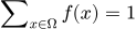
In the case of a discrete random variable X, f is called a probability mass function and the second Kolmogorov axiom is expressed as:
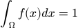
In the case of a continuous random variable X, f is called a probability density function and the second Kolmogorov axiom is expressed as:
Theorems and Properties of Probability
Many important properties of the probability measure derive from the properties of sets. For example
Prob(A) = Prob((A ⋂ B) ⋃ (A ⋂ BC))
Prob(AC ⋂ BC) = Prob((A ⋃ B)C)
Prob(A ⋂ (B ⋃ C)) = Prob((A ⋂ B) ⋃ (A ⋂ C))
Others take advantage of the definition of the probability measure.
Prob(Omega)) = 1 so Prob(A) = 1 - Prob(AC)
A ⊆ B implies Prob(A) ≤ Prob(B)
The probability of a union of disjoint sets is simply the sum of their individual probabilities.
Prob(A ⋃ B) = Prob(A) + Prob(B) for any A,B such that A ⋂ B = Ø
More generally, the probability of a union of 2 events is
Prob(A ⋃ B) = Prob(A) + Prob(B) - Prob(A ⋂ B)
And the probability of a union of 3 events is
Prob(A ⋃ B ⋃ C) = Prob(A) + Prob(B) + Prob(C) - Prob(A ⋂ B) - Prob(B ⋂ C) - Prob(A ⋂ C) + Prob(A ⋂ B ⋂ C)
This generalizes to n events as
\sum \nolimits_i Prob( A_i ) - sum \nolimits_{j<i}n Prob( A_i \cap A_j ) + \sum \nolimits_{k<j<i}n Prob( A_i \cap A_j \cap A_k ) - \dots + (-1){n+1} Prob( \bigcap_{m=1}n A_m)
Joint Probability
In the context of multiple events, the probability of one is called a marginal probability while the probability of an intersection of multiple is called a joint probability. When conceptualizing multiple events, note that they can be sequential or simultaneous without impacting interpretation. This is proven by the equation P(A ∩ B) = P(A|B) P(B) (but more on this below).
As noted above, Prob(A) = Prob((A ⋂ B) ⋃ (A ⋂ BC)) follows immediately from the properties of sets. This is generalized as the law of total probability by considering the sample space to be partitioned by Bi. That is to say, the sample space must be split into n disjoint and exhaustive subsets.
P(A) = \sum_{i=1}^m Prob(A \cap B_i)
The pertains to partitions of a sample space. Let these be notated as Bi. It must be true that
A = (A ⋂ B_i) + (A ⋂ B_i) + ... + (A ⋂ B_i)
Conditional Probability
Generally, the occurrence of one event impacts the probability of another. The intuition is that before event A, our observations existed anywhere in the complete sample space. After the occurrence of A, we have certainty that our observations are not in AC. As such, probabilities must be re-normalized to new domain. That updated probability is expressed as Prob(B|A), or the probability of event B given the occurrence of event A.
Alternatively, consider the probability of A after A has already occurred. Logically it must be that Prob(A|A) = 1 and Prob(AC|A) = 0.
The algebraic definition of a conditional probability is Prob(B|A) = Prob(A ⋂ B) / P(A). A much more common formulation is Prob(A ⋂ B) = Prob(B|A) P(A).
The law of total probability is stated above in terms of joint probabilities, but it is more commonly applied leveraging the above identity.
Prob(A) = \sum_{i=1}^m Prob(A | B_i) Prob(B_i)
See also Bayes' theorem.
Independence
If the occurrence of an event has no impact on the probability of another, then the two events are independent. The direct statement of this identity is Prob(A|B) = Prob(A), but the more useful equation is a statement about the joint probability: Prob(A ⋂ B) = Prob(A) Prob(B).
Independence of two events A and B is notated A ⫫ B.
Conditional independence of two events means that the two events are independent conditioned on some other information. (This 'other information' will henceforth be indicated by a single event C, but generally this refers to a set of predictors.) The direct statement of this identity is Prob(A | B ⋂ C) = Prob(A | C), but the more useful equation is Prob(A ⋂ B | C) = Prob(A | C) Prob(B | C).