|
Size: 932
Comment:
|
Size: 1192
Comment:
|
| Deletions are marked like this. | Additions are marked like this. |
| Line 1: | Line 1: |
| ## page was renamed from 2Equations2Unknowns | |
| Line 20: | Line 21: |
| {{attachment:row-picture.png}} | {{attachment:row-picture.png||width=200}} |
| Line 37: | Line 38: |
| {{attachment:column-picture.png}} | {{attachment:column-picture.png||width=200}} |
| Line 41: | Line 42: |
| {{attachment:column-picture-solution.png}} | {{attachment:column-picture-solution.png||width=200}} == Matrix Picture == {{{ ┌ ┐ ┌ ┐ ┌ ┐ │ 2 -1│ │ x│ │ 0│ │-1 2│ + │ y│ = │ 3│ └ ┘ └ ┘ └ ┘ }}} |
2 Equations, 2 Unknowns
Introduction
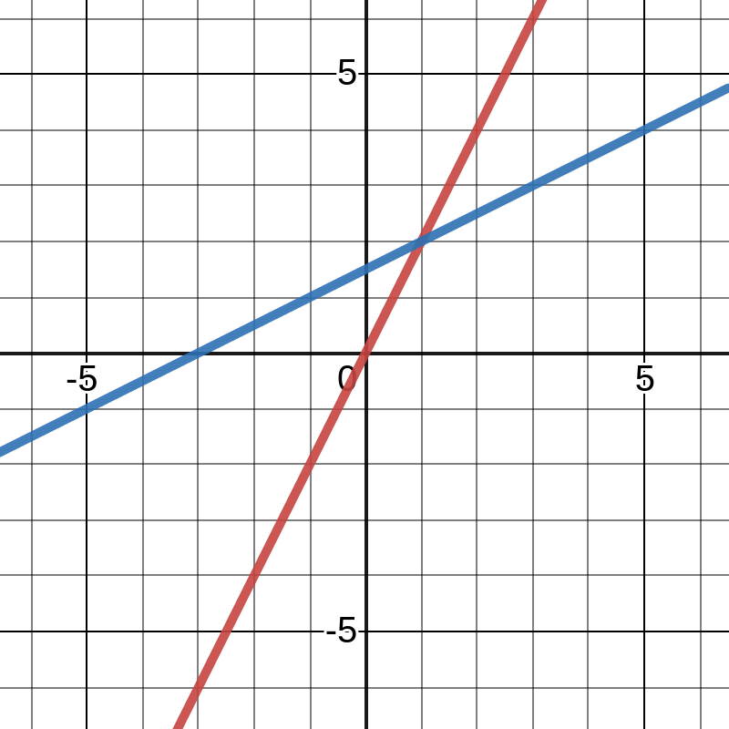
Consider the below system of equations:
2x - y = 0
-x + 2y = 3
This can be envisioned in three ways.
Row Picture
The equations can be plotted together, and all intersections of the lines are solutions to the system.

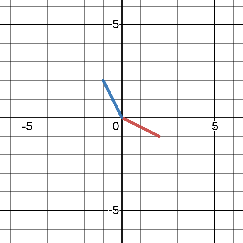
Column Picture
The system is equivalent to the following linear combination of columns.
 ┌  ┐    ┌  ┐   ┌  ┐
 │ 2│    │-1│   │ 0│
x│-1│ + y│ 2│ = │ 3│
 └  ┘    └  ┘   └  ┘
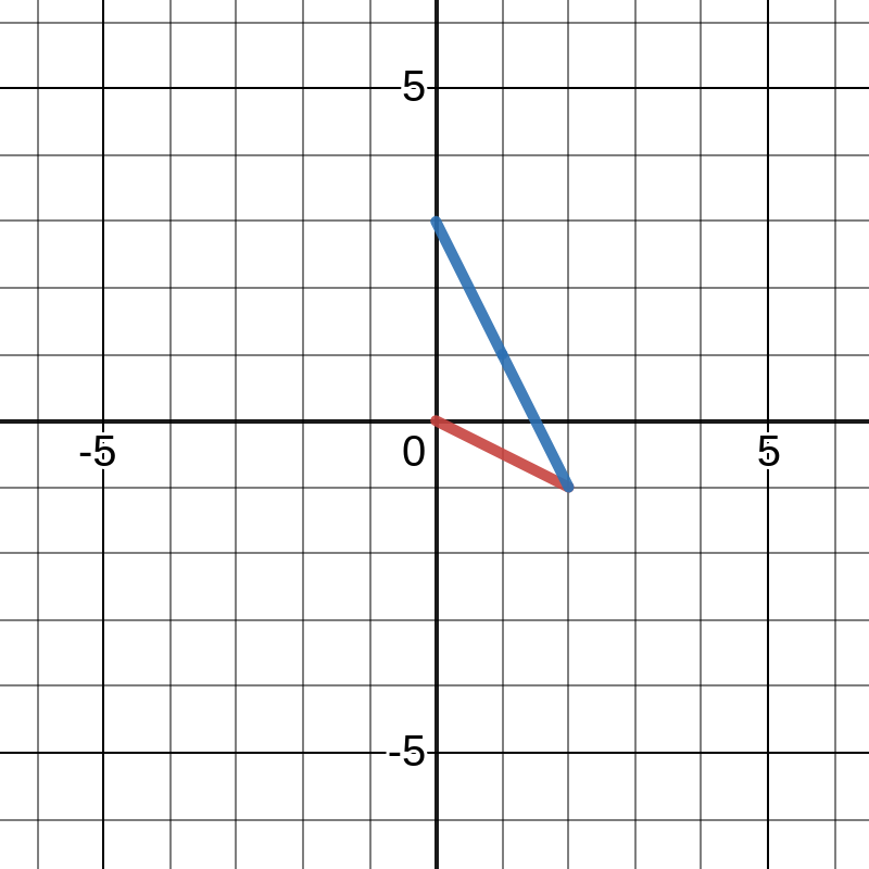
Column 1 is represented as a vector to (2,-1); column 2 as (-1,2).

Any combination of these vectors that leads to (0,3) is a solution to the system. For this system, that solution is 1 of column 1 and 2 of column 2.

Matrix Picture
┌     ┐   ┌  ┐   ┌  ┐
│ 2 -1│   │ x│   │ 0│
│-1  2│ + │ y│ = │ 3│
└     ┘   └  ┘   └  ┘
