Demand Curve
A demand curve relates demand for a good to the price for that good.
Contents
Simple Model
Demand for a good is modeled in terms of other structural factors, such as price of the good, prices of complementary goods, and individual income.
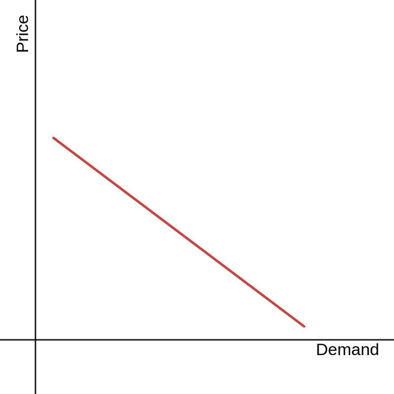
A simple model describes demand (D) in terms of price (P): D = a + bP. This is an example of a demand curve.
Traditionally, the inverse demand curve is graphed instead; that is, price is conceptualized as the dependent variable. The curve is rewritten as P = (D - a)/b.
Interpretation
The above model graphs as:

A demand curve explains how a change in price for some good, holding all else constant, causes a change in demand for that same good. Such a change is called a movement along the curve.
If some other variable is allowed to vary, the demand curve itself changes. This is called a shift of the curve.
Law of Demand
Conventionally, it is assumed that price and demand are inversely related. In the simple model above, this would mean b < 0. In a multivariate model, the assumption looks like ∂D/∂P < 0.
The opposite case is called a Giffen good.
Elasticity
The price elasticity of demand is the rate of relative changes in demand to price. It measures responsivity of a good's demand to price changes while controlling for the price and quantity of the good. This is more useful because a real market consists of n goods and consumer preferences are a dynamic system in terms of each good's price; responsivity must be in common terms across goods.
Arc Elasticity
At it's simplest, elasticity is calculated in reference to two points on a demand curve: (q, p) and (q', p'). Therefore the relative changes used in the rate are computed with:
distance between points (i.e., ΔQ = (q - q') and ΔP = (p - p'))
average of the points (i.e., (q - q')/2 and (p - p')/2)
The notation for arc elasticity is:
Note that sometimes eD is used instead of ε.
Following from the law of demand, elasticity is always negative. Sometimes it is reported as an absolute value.
Point Elasticity
Elasticity can also be differentiated at a point. Partial derivatives are used rather than distances. The point itself is used instead of an average. Lastly, it's helpful to reorganize the terms.
Through the chain rule this can be rewritten as:
Relation to Demand Curves
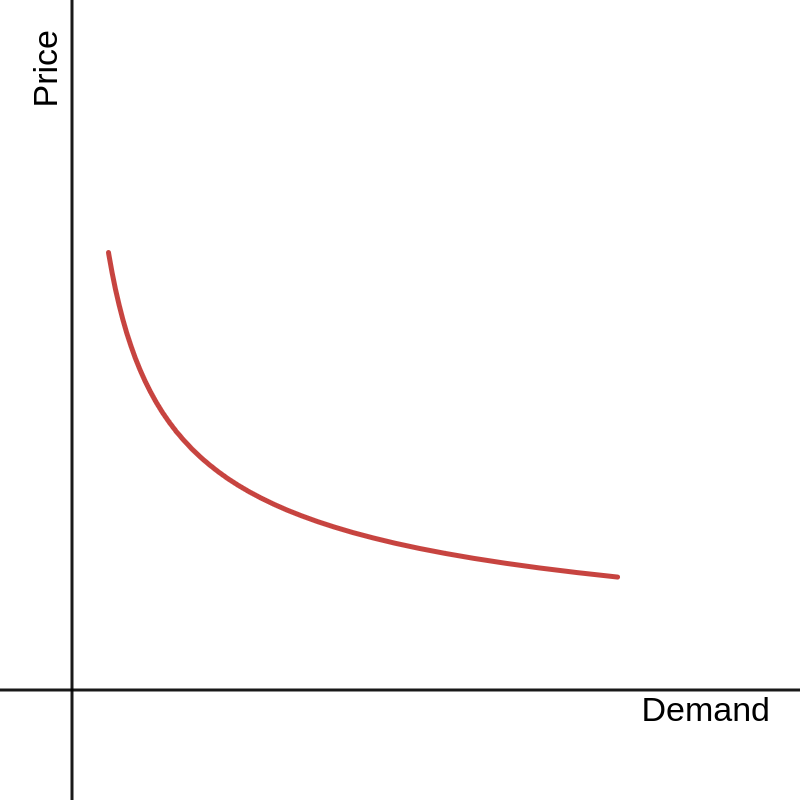
The price elasticity of demand is subtly different from the slope of the demand curve: ∂D/∂P is not a relative rate. The important consequence is that a demand curve with constant elasticity is convex.

If a good is known to have constant elasticity, the demand curve is formulated like D = aPε.
On the contrary, if the demand curve is linear as in the simple model above (i.e., D = a + bP), then elasticity varies in terms of P:
Elasticity is equal to ε = (bp)/(a + bp).
- The demand curve cannot be formulated in terms of elasticity.
There is a point on the demand curve where elasticity is -1; this is called unitary elasticity.
- Above this point, elasticity approaches infinity and the demand curve is price elastic.
- Below this point, elasticity approaches 0 and the demand curve is price inelastic.
Given this, a demand curve featuring constant elasticity is perhaps more plausible and effectively more simple than the 'simple model'.
Perfect inelasticity means demand is unaffected by changes in price. Subsistence or lifesaving goods can be described in this way. Such a good has elasticity of 0; incidentally the demand curve would be drawn as a vertical line (i.e., undefined slope).
Perfect elasticity means price is unaffected by changes in demand. Commodities could be described in this way; regardless of shifts in demand, no seller can succeed in raising prices above the prevailing market price. Such a good has infinite elasticity; incidentally the demand curve would be drawn as a horizonal line (i.e., slope = 0).
