
|
Size: 3104
Comment: Notes
|
← Revision 7 as of 2026-08-11 20:47:13 ⇥
Size: 3274
Comment: Note
|
| Deletions are marked like this. | Additions are marked like this. |
| Line 15: | Line 15: |
| For a random variable ''X'', the variance is usually notated as ''Var(X)''. In contexts where the distribution in question is understood, especially [[Analysis/Error|error]] when analyzing a model, more common notations are ''σ^2^'' for population variance or ''s^2^'' for sample variance. (This enables notation like ''s,,i,,^2^'', for the variance of errors for observation ''i''.) | For a random variable ''X'', the variance is usually notated as ''Var(X)'' or ''Var[X]''. In contexts where the distribution in question is understood, ''σ^2^'' is commonly used. If a particular distribution function can be assumed, there may be a simple formula for variance. For example: * for a [[Analysis/BernoulliDistribution|Bernoulli distribution]], ''p(1-p)'' * for a [[Analysis/BinomialDistribution|Binomial distribution]], ''np(1-p)'' * for a [[Analysis/PoissonDistribution|Poisson distribution]], ''λ'' * for a [[Analysis/UniformDistribution|Uniform distribution]], ''(b-a)^2/12'' * and so on... The variance of a random vector X is a [[Analysis/Covariance|covariance matrix]]. === Properties === If the variance of a random variable ''X'' is known, adding a constant to ''X'' does not change the variance. Multiplying ''X'' by a constant factor scales the known variance by the square of the factor. Succinctly: ''Var(aX + b) = a^2^ Var(X)'' The inverse of variance is called '''precision'''. === Estimation === In most circumstances, [[Statistics/SamplingDistribution|sample variance]] (notated ''s^2^'') is an unbiased estimator for the true variance ''σ^2^''. The exceptions are distributions with an undefined expected value or infinite variance, like the [[Analysis/CauchyDistribution|Cauchy distribution]]. Furthermore there are circumstances where the estimate should not be considered good, as with small sample sizes. When working with a set of observations ''X'', where for each observation ''i'' there is an observed value ''x,,i,,'', sample variance is calculated as: {{attachment:samp.svg}} |
| Line 23: | Line 50: |
| Formally, the second central moment (implicitly taking the [[Analysis/ExpectedValue|expected value]] as the center) of a continuous quantitative random variable is: | Formally, the second central moment (implicitly taking the [[Analysis/ExpectedValue|expected value]] as the center) of a continuous quantitative (numeric) random variable is: |
| Line 35: | Line 62: |
| But when working with a set of observations ''X'', where for each observation ''i'' there is an observed value ''x,,i,,'', the most common formulas for variance are: | Variance is therefore an expected value: |
| Line 37: | Line 64: |
| {{attachment:var.svg}} | {{attachment:exp1.svg}} |
| Line 39: | Line 66: |
| To get from the first to the second, the derivation for discrete variables is: | By completing the square and spreading the expected value function, a simpler formula is derived. Note that expectations are linear (i.e., ''E[a + b] = E[a] + E[b]'') and that the expected value of an expected value is the expected value itself (i.e., ''E[E[a]] = E[a]''). |
| Line 41: | Line 68: |
| * ''Σ (x - μ)^2^ P(x=X)'' * ''Σ (x^2^ - 2μx + μ^2^) P(x=X)'' * ''Σ [x^2^ P(x=X)] - 2μ Σ [x P(x=X)] + μ^2^ Σ [P(x=X)]'' * ''[E[X^2^]] - 2μ [μ] + μ^2^ [1]'' * ''E[X^2^] - 2μ^2^ + μ^2^'' * ''E[X^2^] - μ^2^'' * ''E[X^2^] - (E[X])^2^'' The derivation for continuous variables is: * ''∫ (x - μ)^2^ f(x) dx'' * ''∫ (x^2^ - 2μx + μ^2^) f(x) dx'' * ''∫ [x^2^ f(x) dx] - 2μ ∫ [x f(x) dx] + μ^2^ ∫ [f(x) dx]'' * ''[E[X^2^]] - 2μ [μ] + μ^2^ [1]'' * ''E[X^2^] - 2μ^2^ + μ^2^'' * ''E[X^2^] - μ^2^'' * ''E[X^2^] - (E[X])^2^'' (Recall that definitionally, ''1 = ∫ f(x) dx'' for any probability density function.) It should also be clear that you can pick out the formulation as ''Var(X) = Σ(X^2^)/n - (E[X])^2^'', which can be useful in certain situations. ---- == Variance as a Function == If the variance of a random variable ''X'' is known, adding a constant to ''X'' does not change the variance. Multiplying ''X'' by a constant factor scales the known variance by the square of the factor. Succinctly: ''Var(aX + b) = a^2^ Var(X)'' The variance of a ratio, i.e. ''Var(X/Y)'' where both ''X'' and ''Y'' are variable, is nonlinear. |
{{attachment:exp2.svg}} |
Variance
Variance is a measure of dispersion or spread. It is the second central moment.
Contents
Description
Variance is measure of how much observations vary from the expected value. If the expected value is expressed in 'units', then variance is expressed in 'units squared'. This can pose challenges to interpretation, so a closely related statistic is the standard deviation: the square root of variance.
For a random variable X, the variance is usually notated as Var(X) or Var[X]. In contexts where the distribution in question is understood, σ2 is commonly used.
If a particular distribution function can be assumed, there may be a simple formula for variance. For example:
for a Bernoulli distribution, p(1-p)
for a Binomial distribution, np(1-p)
for a Poisson distribution, λ
for a Uniform distribution, (b-a)^2/12
- and so on...
The variance of a random vector X is a covariance matrix.
Properties
If the variance of a random variable X is known, adding a constant to X does not change the variance. Multiplying X by a constant factor scales the known variance by the square of the factor. Succinctly: Var(aX + b) = a2 Var(X)
The inverse of variance is called precision.
Estimation
In most circumstances, sample variance (notated s2) is an unbiased estimator for the true variance σ2. The exceptions are distributions with an undefined expected value or infinite variance, like the Cauchy distribution. Furthermore there are circumstances where the estimate should not be considered good, as with small sample sizes.
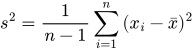
When working with a set of observations X, where for each observation i there is an observed value xi, sample variance is calculated as:
Formulation
Formally, the second central moment (implicitly taking the expected value as the center) of a continuous quantitative (numeric) random variable is:

where Ω is the sample space and f is the probability density function for that distribution.
And for a discrete quantitative random variable:

where Ω is the set of possible values and f is the probability mass function for that distribution (although the distributions of discrete random variables are commonly given as tables, rather than mathematical functions).
Variance is therefore an expected value:

By completing the square and spreading the expected value function, a simpler formula is derived. Note that expectations are linear (i.e., E[a + b] = E[a] + E[b]) and that the expected value of an expected value is the expected value itself (i.e., E[E[a]] = E[a]).
