
|
Size: 975
Comment: Initial commit
|
Size: 3896
Comment: MLE
|
| Deletions are marked like this. | Additions are marked like this. |
| Line 3: | Line 3: |
| The '''normal distribution''' is a bell-shaped continuous probability distribution that is parameterized to a mean and standard deviation. | The '''normal distribution''' is a bell-shaped continuous probability distribution function that is parameterized to a mean and standard deviation. |
| Line 13: | Line 13: |
| The distribution is bell-shaped. | The distribution is bell-shaped and parameterized to the [[Analysis/Moment|first and second central moments]]. This has useful consequences for estimating the probability that a given value is in the distribution. For example: |
| Line 17: | Line 18: |
A variable distributed this way is notated like ''X ~ N(μ, σ^2^)''. The probability density function is given (and commonly notated) as: {{attachment:norm.svg}} Correspondingly, the cumulative probability function is commonly notated as ''Φ(.)'' rather than ''F(.)''. Furthermore the quantile function is commonly notated as ''Φ^-1^(.)''. === Standard Normal Distribution === The '''standard normal distribution''' is specified as ''Z ~ N(0, 1)''. Compare to the calculation for '''Z scores''' that will be compared to the standard normal distribution: ''Z = (x - μ)/σ''. The probability density function simplifies to: {{attachment:stdnorm.svg}}. This is graphed as: {{attachment:stdnormgraph.png||width=300px}} |
|
| Line 22: | Line 47: |
| == Statistics == | == Moments == |
| Line 24: | Line 49: |
| The mean and standard deviation are necessarily given by the distribution formulation. | The [[Analysis/ExpectedValue|expected value]] is given as ''E[X] = μ''. [[Analysis/Variance|Variance]] is given as ''Var[X] = σ^2^''. ---- == Estimation == The [[Statistics/MaximumLikelihood|MLE]] for ''μ'' is ''X̅''. This is derived as: {{attachment:mu1.svg}} {{attachment:mu2.svg}} Now applying log properties: {{attachment:mu3.svg}} And now pulling all constants out of summations: {{attachment:mu4.svg}} The critical points of this equation are found by deriving with respect to ''μ''. The first part of the RHS is a constant with respect to ''μ'' to becomes 0. {{attachment:mu5.svg}} {{attachment:mu6.svg}} Multiply both sides by ''σ^2^'' and add ''nμ'' to both sides to get: {{attachment:mu7.svg}} Finally, recognize that ''X̅ = (1/n) Σ,,i,,(x,,i,,)''. Therefore ''μ,,MLE,, = X̅''. |
| Line 34: | Line 93: |
| === Standard Normal Distribution === | === Normality of Sampling Distributions === |
| Line 36: | Line 95: |
| The normal distribution characterized by a mean of 0 and a standard deviation of 1 is called the '''standard normal distribution'''. This distribution is referenced for '''Z scores''' (alternatively called '''Z statistics'''). | For a population parameter whose population distribution is normal with mean ''μ'' and variance ''σ^2^'', the sampling distribution of the sample statistic which estimates that parameter is also normal. In particular, ''X̅'' is the sample statistic that estimates ''μ'', and its sampling distribution is normal with mean ''X̅ = μ'' and variance ''σ^2^,,X̅,, = σ^2^,,X,,/n'', where ''n'' is the sample size. By the central limit theorem, even when the population distribution in question is '''not''' normal, with a sufficiently large sample size the sampling distribution of the sample statistic which estimates that parameter '''is'''. A note on variance of a sampling distribution (i.e., ''σ^2^,,X̅,,'' not ''σ^2^,,X,,''). This is a function of both the sample variance ''σ^2^,,X,,'', which is usually itself estimated using sample variance (i.e., ''σ^2^,,X,, = s^2^,,X̅,,''), and the sample size ''n''. Consider a census of the population; there is only one possible sample so the sampling distribution has only a single level with 100% certainty. As the sample size decreases, the number of possible samples grows. The number of levels in the sampling distribution is also expected to grow accordingly. === Probability Tests === As noted above, '''Z scores''' (alt. ''Z statistics'') are test statistics for which likelihood can be calculated using the standard normal distribution. |
Normal Distribution
The normal distribution is a bell-shaped continuous probability distribution function that is parameterized to a mean and standard deviation.
Contents
Description
The distribution is bell-shaped and parameterized to the first and second central moments. This has useful consequences for estimating the probability that a given value is in the distribution. For example:
- 68.27% of the cumulative distribution is within 1 standard deviation of the mean
- 95.45% within 2
- 99.73% within 3
A variable distributed this way is notated like X ~ N(μ, σ2).
The probability density function is given (and commonly notated) as:

Correspondingly, the cumulative probability function is commonly notated as Φ(.) rather than F(.). Furthermore the quantile function is commonly notated as Φ-1(.).
Standard Normal Distribution
The standard normal distribution is specified as Z ~ N(0, 1).
Compare to the calculation for Z scores that will be compared to the standard normal distribution: Z = (x - μ)/σ.
The probability density function simplifies to:
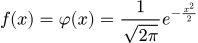 .
.
This is graphed as:

Moments
The expected value is given as E[X] = μ.
Variance is given as Var[X] = σ2.
Estimation
The MLE for μ is X̅. This is derived as:


Now applying log properties:

And now pulling all constants out of summations:

The critical points of this equation are found by deriving with respect to μ. The first part of the RHS is a constant with respect to μ to becomes 0.
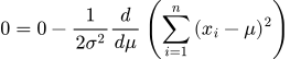

Multiply both sides by σ2 and add nμ to both sides to get:

Finally, recognize that X̅ = (1/n) Σi(xi). Therefore μMLE = X̅.
Usage
Normality of Sampling Distributions
For a population parameter whose population distribution is normal with mean μ and variance σ2, the sampling distribution of the sample statistic which estimates that parameter is also normal. In particular, X̅ is the sample statistic that estimates μ, and its sampling distribution is normal with mean X̅ = μ and variance σ2X̅ = σ2X/n, where n is the sample size.
By the central limit theorem, even when the population distribution in question is not normal, with a sufficiently large sample size the sampling distribution of the sample statistic which estimates that parameter is.
A note on variance of a sampling distribution (i.e., σ2X̅ not σ2X). This is a function of both the sample variance σ2X, which is usually itself estimated using sample variance (i.e., σ2X = s2X̅), and the sample size n. Consider a census of the population; there is only one possible sample so the sampling distribution has only a single level with 100% certainty. As the sample size decreases, the number of possible samples grows. The number of levels in the sampling distribution is also expected to grow accordingly.
Probability Tests
As noted above, Z scores (alt. Z statistics) are test statistics for which likelihood can be calculated using the standard normal distribution.
As an example, for a two-tailed test and a significance level of 5%, the critical Z score value is 1.96.