
|
Size: 2761
Comment: Initial commit
|
← Revision 5 as of 2026-08-11 18:16:42 ⇥
Size: 3978
Comment: Notes
|
| Deletions are marked like this. | Additions are marked like this. |
| Line 23: | Line 23: |
| The expected value of a random vector ''X'' is equal to the expected value of each member. This should make clear that the expected value is a vector of equal dimensions to the random vector itself. === Estimation === Definitionally, [[Statistics/SamplingDistribution|sample mean]] ''X̅'' is '''always''' an unbiased estimator for the expected value ''E[X]'', '''unless''' the distribution has no defined expected value at all (e.g. the [[Analysis/CauchyDistribution|Cauchy distribution]]). The standard error of that estimator is a function of the population distribution's [[Analysis/Variance|variance]] and the sample size: ''σ^2^,,X̅,, = σ^2^,,X,,/n''. === Properties === Expectations are linear. If the expected value of a random variable ''X'' is known, adding a constant to ''X'' also adds that constant to the expected value. Multiplying ''X'' by a constant factor also multiplies the known variance by that factor. Succinctly: ''E[aX + b] = a E[X] + b''. This holds for linear transformations of random vectors. Let ''x'' be a random vector of size ''n x 1'', ''b'' be a constant vector of the same size, and ''A'' be a constant matrix of size ''m x n''. Given these, ''E[Ax + b] = A E[x] + b''. The expected value of the sum of two random variables (or vectors) ''X'' and ''Y'' is the sum of their expected values: ''E[X + Y] = E[X] + E[Y]''. Similarly, if two random variables (or vectors) are independent, then the expected value of their product is the product of their expected values: ''E[XY] = E[X]E[Y]''. Also consider the ratio of two independent random variables: ''E[X/Y] = E[X]E[1/Y]''. Note that this is ''not'' equivalent to ''E[X]/E[Y]''. |
|
| Line 41: | Line 65: |
| But when working with a set of observations ''X'', where for each observation ''i'' there is an observed value ''x,,i,,'', and for which there is a function ''p'' describing the probability of ''X'' taking on the value ''x,,i,,'' (sometimes expressed as ''p(X=x)''), the most common formula is: | When working with a distribution given as a table, pairing values of ''X'' with a known probability (i.e. there is a function ''p'' describing the probability of ''X'' taking on the value ''x,,i,,''), the most common formulation is: |
| Line 43: | Line 67: |
| {{attachment:exp.svg}} | {{attachment:exp1.svg}} |
| Line 45: | Line 69: |
| ---- | When working with a set of observations ''X'', where for each observation ''i'' there is an observed value ''x,,i,,'', the most common formula is: |
| Line 47: | Line 71: |
| {{attachment:exp2.svg}} | |
| Line 48: | Line 73: |
== Expected Value as a Function == Expectations are linear. If the expected value of a random variable ''X'' is known, adding a constant to ''X'' also adds that constant to the expected value. Multiplying ''X'' by a constant factor also multiplies the known variance by that factor. Succinctly: ''E[aX + b] = a E[X] + b''. The expected value of the sum of two random variables ''X'' and ''Y'' is the sum of their expected values: ''E[X + Y] = E[X] + E[Y]''. Similarly, if two random variables are independent, then the expected value of their product is the product of their expected values: ''E[XY] = E[X]E[Y]''. This is not true if the two are related; refer to the common formula for covariance: ''Cov(X, Y) = E[XY] - E[X]E[Y]''. Also consider the ratio of two independent random variables: ''E[X/Y] = E[X]E[1/Y]''. Note that this is ''not'' equivalent to ''E[X]/E[Y]''. |
This can be equivalently expressed using a ones-vector ''j''. Let ''x'' be the vector of observed values: * ''(x⃗ · ĵ) 1/n'' * ''(x^T^j) 1/n'' for a more [[LinearAlgebra|linear algebraic]] formulation * ''(x^T^Ij) 1/n'' to look more like a [[LinearAlgebra/QuadraticForm|quadratic form]] |
Expected Value
The expected value of a random variable is its average, i.e. the value that can be assumed for a finite set of observations without impacting the sum.
Description
For a random variable X, the expected value is usually notated as E[X], E(X), X̅.
More commonly though, a particular distribution function is assumed and the expected value is written in terms appropriate for the corresponding first moment. For example:
for a Normal distribution, μ
for a Bernoulli distribution, p
for a Binomial distribution, np
for a Poisson distribution, λ
for a Uniform distribution, (a+b)/2
- and so on...
The expected value of a random vector X is equal to the expected value of each member. This should make clear that the expected value is a vector of equal dimensions to the random vector itself.
Estimation
Definitionally, sample mean X̅ is always an unbiased estimator for the expected value E[X], unless the distribution has no defined expected value at all (e.g. the Cauchy distribution).
The standard error of that estimator is a function of the population distribution's variance and the sample size: σ2X̅ = σ2X/n.
Properties
Expectations are linear. If the expected value of a random variable X is known, adding a constant to X also adds that constant to the expected value. Multiplying X by a constant factor also multiplies the known variance by that factor. Succinctly: E[aX + b] = a E[X] + b.
This holds for linear transformations of random vectors. Let x be a random vector of size n x 1, b be a constant vector of the same size, and A be a constant matrix of size m x n. Given these, E[Ax + b] = A E[x] + b.
The expected value of the sum of two random variables (or vectors) X and Y is the sum of their expected values: E[X + Y] = E[X] + E[Y].
Similarly, if two random variables (or vectors) are independent, then the expected value of their product is the product of their expected values: E[XY] = E[X]E[Y].
Also consider the ratio of two independent random variables: E[X/Y] = E[X]E[1/Y]. Note that this is not equivalent to E[X]/E[Y].
Formulation
Formally, the first moment of a continuous quantitative (numeric) random variable is:

where Ω is the sample space and f is the probability density function for that distribution.
And for a discrete quantitative random variable:

where Ω is the set of possible values and f is the probability mass function for that distribution (although the distributions of discrete random variables are commonly given as tables, rather than mathematical functions).
When working with a distribution given as a table, pairing values of X with a known probability (i.e. there is a function p describing the probability of X taking on the value xi), the most common formulation is:

When working with a set of observations X, where for each observation i there is an observed value xi, the most common formula is:
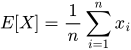
This can be equivalently expressed using a ones-vector j. Let x be the vector of observed values:
(x⃗ · ĵ) 1/n
(xTj) 1/n for a more linear algebraic formulation
(xTIj) 1/n to look more like a quadratic form